Specimen Section 1
You are a public health advisor in an inner city community within a large metropolitan area of a developed country. In recent years, a ‘congestion charge’ has been introduced which requires drivers of private vehicles to pay a daily fee for driving into the city centre. Traffic census data indicate that this has resulted in a 20% decline in car and light van traffic within the congestion charge zone. The following statistics have been compiled from one of the primary care health centres situated within the congestion charge zone:
| Patients attending the primary care centre for asthma during: | |||
| 12 months before the congestion charge was introduced | 450 | ||
| 12 months after the congestion charge was introduced | 500 | ||
| Primary care consultations for acute asthma attacks during: | |||
| 12 months before the congestion charge was introduced | 175 | ||
| 12 months after the congestion charge was introduced | 125 | ||
Questions
(a) What further single item of information would you require to estimate the annual period prevalence of asthma in this area, after the introduction of the congestion charge zone? (1 mark)
(b) Describe and calculate a suitable measure for comparing the occurrence of acute asthma attacks before and after the introduction of the congestion charge. (2 marks)
(c) State two assumptions you have used in your calculation in (b). (2 marks)
(d) Calculate an appropriate statistical test to determine whether the change in incidence of acute asthma attacks around the time of introduction of the congestion charge was statistically significant at the 5% level. (3 marks)
(e) Write no more than four sentences for inclusion in your public health department’s annual report, summarising your conclusions regarding the effect of the congestion charge policy on the burden of asthma locally. (2 marks)
Specimen Section 2
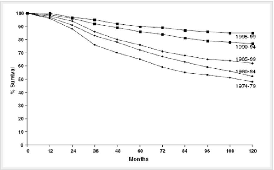
Results relating to the survival of successive cohorts of women diagnosed with breast cancer were recently published from a Western European country and are illustrated in the figure. A national programme of breast cancer screening was introduced in 1989.
Figure. Breast cancer specific survival in 5-year cohorts defined by date of diagnosis between 1974 and 1999
Questions
(a) Choose the single answer that best defines “breast cancer specific survival” (1 mark)
A: The proportion of women who survive for a specified period without developing breast cancer.
B: The proportion of breast cancer patients who survive for a specified period after their date of diagnosis.
C: The proportion of breast cancer patients who survive for a specified period after the date of diagnosis with breast cancer, or whose cause of death is not certified as breast cancer.
D: The proportion of breast cancer patients who survive for a specified period after the date of diagnosis with breast cancer, or who die from non-accidental causes.
E: The proportion of breast cancer patients who survive for a specified period relative to the proportion of the general population of a similar age who survive for the same period.
(b) Give three possible explanations for the larger change between the 1985-1989 and the 1990-1994 cohorts compared with that between the other cohorts. (3 marks)
(c) Describe two other important features of the data shown in the figure. (2 marks)
Further survival information is provided in the table below.
Table. Overall survival (%) in the 1980-1984 and 1990-1994 diagnostic cohorts at 5, 10 and 15 years of follow-up
| % Survival at: | 1980-1984 | 1990-1994 | Proportional risk reduction |
| 5 years | 73 | 88 | 0.56 |
| 10 years | 55 | 80 | 0.56 |
| 15 years | 46 | 78 | 0.59 |
(d) What does the term ‘proportional risk reduction’ mean and how was it calculated? (2 marks)
(e) Write no more than four sentences for inclusion in a press release to your local newspaper, summarising the findings given in the table above, and their interpretation. (2 marks)
Specimen Section 3
Results were recently published from a register of visual impairment in childhood in a developed country. Only children notified up to the age of 10 years were eligible for inclusion on the register. Between 1984 and 1998, a total of 691 children with visual impairment were notified to the register (see table below), of whom 130 have subsequently died, with 58% dying before they reached their fifth birthday.
Table. Characteristics of the children with any degree of visual impairment (moderate, severe or blind) born between 1984 and 1998
| Number of cases on the register n=691 | Number of live births in the catchment population n=520,240 | |
| Singleton or multiple birth: | ||
| Multiple | 35 | 13,239 |
| Singleton | 656 | 507,001 |
| Sex of child: | ||
| Male | 415 | 266,542 |
| Female | 276 | 253,698 |
Questions
(a) Calculate the overall case fatality of childhood visual impairment. (1 mark)
(b) Calculate the cumulative incidence ratio for any degree of visual impairment in males compared with females. (2 marks)
(c) The cumulative incidence ratio for multiple births compared to singleton births is 2.0 (95% confidence interval 1.5 to 2.9). In no more than three sentences, explain what this statement means and comment on the statistical significance of this result. (3 marks)
The results from this analysis of registered cases were compared with data from a cross-sectional study of children whose visual acuity was measured when they were 10 years old. Assuming that both sets of data are representative of the same national population:
(d) Explain in one or two sentences how and why the two sets of results might differ in their estimate of the incidence of blindness? (2 marks)
(e) Explain in one or two sentences how and why the two sets of results might differ in their estimate of the incidence of moderate visual impairment? (2 marks)
Specimen Section 4
Your healthcare organisation is providing funding for the drug trastuzumab for the treatment of HER2 positive cases of breast cancer. This costs £25,000 per course of treatment. Testing of breast cancer tissue to determine HER2 status involves the use of immuno-histochemistry (IHC) which is a tissue stain test, and/or fluorescent in situ hybridisation (FISH) which is a genetic test. Your healthcare organisation currently uses IHC which costs £40 per test. FISH is more expensive at £150 per test but is less prone to observer variation.
You have been asked to conduct a review and report on the implications of different testing regimens. For the purposes of your review all the breast cancer biopsy specimens tested during one year were subjected to FISH testing in addition to IHC. The results are shown in the table below.
Table. Annual number of biopsy specimens by immuno-histochemistry (IHC) category and proportion of FISH positive results within each IHC category
| Immuno-histochemistry result | Number of biopsies from your local laboratory with this IHC result | Percentage of positive FISH results for biopsies within each IHC category |
| Negative | 22,500 | 1% |
| Weakly positive | 3,600 | 50% |
| Strongly positive | 3,900 | 94% |
The current policy is that all women with "strongly positive" IHC results are offered treatment with trastuzumab.
Questions
(a) Assuming that FISH is the reference (gold) standard for HER2 positivity, what is the positive predictive value of a "strongly positive" IHC result? (1 mark)
(b) Compare the cost of performing FISH tests on all "strongly positive" IHC specimens with the saving in treatment costs that would be expected from applying this 2-step approach. (2 marks)
(c) Assuming that FISH is the reference (gold) standard for HER2 positivity, calculate the sensitivity of the test programme to detect HER2 positive cases if:
(i) Only "strongly positive" IHC results are considered test positive (1 mark)
(ii) Both "strongly positive" and "weakly positive" IHC results are considered test positive (1 mark)
(iii) All specimens are tested by FISH instead of IHC (1 mark)
(d) Assuming FISH is the gold standard for HER2 positivity, calculate the marginal test-associated cost of identifying one HER2 positive case if all specimens were tested by FISH, instead of the current policy of testing all specimens by IHC and treating only those that are strongly IHC positive. (3 marks)
(e) What single additional piece of information would be most important to complete an economic evaluation of whether to test all specimens by FISH, instead of IHC? (1 mark)
Specimen Section 5:
You are the public health advisor to a local government authority responsible for municipal services for 200,000 people. Concerns were raised at a recent public meeting about two recent reports in the medical literature, suggesting that swimming in indoor chlorinated pools may increase the risk of asthma in children.
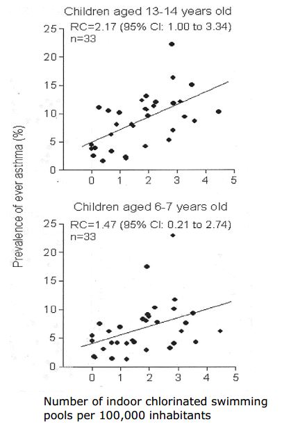
The first report correlated the lifetime prevalence of asthma, as reported by parental questionnaire in surveys of schoolchildren in two age groups, with the number of public indoor chlorinated swimming pools per 100,000 inhabitants in 33 towns and cities throughout Europe (Figure 1).
Figure 1: Lifetime prevalence of asthma in children of two age groups in relation to the number of indoor chlorinated swimming pools in 33 centres
across Europe.
(RC = regression coefficient, 95%CI = 95% confidence interval) Number of indoor chlorinated swimming pools per 100,000 inhabitants
(a) What type of epidemiological study design is this? (1 mark)
(b) In 2-4 sentences, interpret the regression coefficient and its 95%CI in the upper graph. (2 marks)
(c) In 2-4 sentences, compare the findings in the two age groups. (2 marks)
(d) Suggest two pieces of further information about this study that would aid in the interpretation of these findings. (2 marks)
The second report, by the same authors, compared 43 children who had followed a programme of infant swimming lessons before 2 years of age,
with the remaining 298 children in a cross-sectional survey of 10-yearolds in suburban Brussels. The lifetime prevalences of asthma in the two groups were 23.3% (10/43) and 11.1% (33/298), respectively.
(e) Perform an appropriate test to evaluate the statistical significance of the association of infant swimming with asthma in this second study. (3 marks)
Specimen Section 6:
A recent television series presented by a celebrity chef has excited a local and national debate about the nutritional adequacy of school meals. You are the public health advisor for a large town that has a number of schools providing education for 20,000 school children (aged 5-18 years). In response to local media interest, the education department has linked records of school meal purchases to the results of a recent routine survey of the heights and weights of children in their final year at primary school (age 10-11 years) throughout the town. The education department has asked your advice about interpretation of these data.
| School meals eaten daily? | Number of children | Percentage of boys | Mean (SD) Height (cm) |
Mean (SD) Weight (kg) |
| Yes | 1437 | 45% | 140.9 (7.6) | 35.4 (9.0) |
| No | 510 | 54% | 140.5 (7.5) | 34.5 (9.2) |
(a) Calculate a measure of the difference in body weight between the children who eat school meals daily and the remaining children, and its 95% confidence interval. Comment on your finding. (3 marks)
(b) In 2-3 sentences, comment on the likely effect of adjusting these comparisons for the sex of the children. (3 marks)
(c) Suggest and justify one additional factor that it would be important to adjust for. (1 mark)
(d) In up to 3 sentences, outline a more statistically powerful study design, for comparing the body composition of children grouped according to consumption of school meals. (3 marks)
Specimen Section 7:
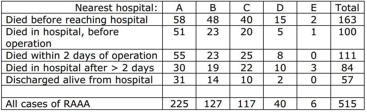
A review of all cases of ruptured abdominal aortic aneurysm (RAAA) (a life threatening condition) over the past 4 years in a predominantly rural area identified 515 cases. The following table shows the frequency of each outcome in relation to the nearest hospital. All of the patients who reached hospital alive were treated at the hospital nearest to their home. Patients who died before reaching hospital were classified by the hospital nearest their home.
(a) List four sources of information that might be used to ascertain all cases of RAAA in the area. (2 marks)
(b) What problems might arise in determining the number of incident cases of RAAA? (2 marks)
(c) From the information in the table, evaluate and comment upon the relationship between volume of emergency RAAA repair and postoperative survival. (4 marks)
Travel times from each patient’s home to the nearest hospital were estimated. After adjustment for age, sex, deprivation score, and nearest hospital, the odds ratio of survival to hospital discharge after RAAA was calculated as 0.97 (95% confidence interval 0.70-1.34) per 10 minutes additional travelling time. Recalculating travel times for each RAAA patient, on the assumption that all cases were transported immediately to a centralised vascular surgery service at hospital A, resulted in an average increase in travelling time from home to hospital of 20 minutes.
(d) Estimate the likely impact of an additional 20 minutes average travelling time upon the odds of surviving RAAA. (2 marks)
| Please note that specimen questions 9 and 10 have been taken down for clarification and review. |
Specimen section 8
Data were obtained from the investigation of an outbreak of E. coli O157 infection among children attending a nursery.
Figure 1 shows the epidemic curve for all nursery children who were either laboratory-confirmed cases or who met an appropriate epidemiological case definition.
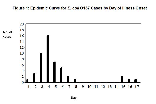
(a) What likely mode of transmission of infection do the data in figure 1 indicate? (2 marks)
Table 1 shows the foodstuffs that nursery staff reported having served to the nursery children two days before the onset of illness in the index case.
Table 1: Foodstuffs Served to Children Two Days Prior to Day of Onset of Illness in Index Case
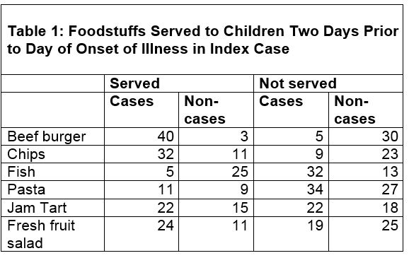
(b) From Table 1, calculate the attack rate for those served beef burger. (1 mark)
(c) Perform an appropriate statistical test to determine whether or not the difference in attack rate for those served or not served beef burger is statistically significant. (3 marks)
(d) Further analysis shows that the associations between being served chips or fresh fruit salad and being a case are statistically significant. What four more pieces of information may help you assess whether beef burger, fruit salad or chips was the most likely outbreak vehicle? (4 marks)
Specimen Section 9
A law to ban tobacco smoking in all enclosed public places and workplaces was introduced into a north European country on 1st April 2006. Researchers collected information about the number of admissions to hospital for heart attack for the six months before the introduction of the new law and for the six months after the introduction (Table 2).
|
Table 2: Number of patients admitted with heart attack by smoking status before and after the introduction of the smoking-ban law |
||
|
|
Number of admissions with heart attack |
|
|
|
Total population: 10,000 |
Total population: 10,000 |
|
|
Period 1 – before new law introduced |
Period 2 - after new law introduced |
|
Current smokers |
1176 |
1016 |
|
Former smokers |
953 |
769 |
|
Never smokers |
677 |
537 |
(a) Separately, for current smokers and for never smokers, calculate the relative risk reduction in admissions for heart attack for the period after the introduction of the law banning smoking compared with the period before. (2 marks)
(b) Describe (but do not calculate) what test(s) you might undertake in order to establish whether the different relative risk reduction in admissions for heart attack among current smokers and never smokers was likely to be due to chance. (2 marks)
Overall there was a 17% reduction in the number of patients admitted with heart attack after the introduction of the new law; this result was statistically significant. One possible explanation for the overall reduction in the number of patients admitted with heart attack was the effect of the new law banning smoking.
(c) State, in no more than four sentences, two other possible reasons for this reduction. (2 marks)
(d) Assuming that the new law was effective in reducing smoking in public places, describe, in one sentence, a potential adverse public health effect of this reduction. (1 mark)
As part of this study, the researchers monitored serum cotinine levels in the general population and in the people admitted to hospital with heart attack.
(e) Cotinine levels in the general population decreased significantly, whereas there was no reduction in cotinine levels in smokers admitted to hospital with heart attack. Explain in no more than three sentences why this might be the case. (3 marks)
Specimen Section 10
Associations between childhood immunisation and all-cause childhood mortality have been reported. Table 3 shows data from a prospective cohort study on child survival according to BCG vaccination status before age two years, conducted in a developing country. The study collected information on 9085 children born in the study area between 1985 and 1993. Researchers visited the families on average every six months. Follow-up stopped after either death or migration out of the study area. The mean age at which children received BCG vaccine was 4.8 months. Evidence of BCG vaccination was based on written entry in parent-held immunisation records. At death it is routine practice in the study area to discard all of the child’s belongings and any such parent-held health records.
|
Table 3: Rate ratios for mortality before age two years and BCG immunisation by vaccination status |
||
|
|
Deaths from all causes (person-months at risk) |
Mortality rate ratio (95% confidence interval) |
|
Unadjusted: |
|
|
|
Unvaccinated |
958 (72938) |
1.00 |
|
Given BCG |
64 (14238) |
0.37 (0.29-0.48) |
|
Adjusted*: |
|
|
|
Unvaccinated |
953 (72410) |
1.00 |
|
Given BCG |
63 (14200) |
0.37 (0.27-0.50) |
* Adjusted for area, dispensary in village, frequent family use of health services, diarrhoea during first year of life and birth season.
(a) Summarise the findings of the data in Table 3. (3 marks)
(b) Suggest two possible reasons why adjustment for covariates did not alter the mortality ratio. (2 marks)
(c) Describe two major biases arising from the design of this. (4 marks)
(d) What other study design could have been used to test whether or not there are non-specific benefits on mortality from BCG vaccination? (1 mark)
Specimen Section 11
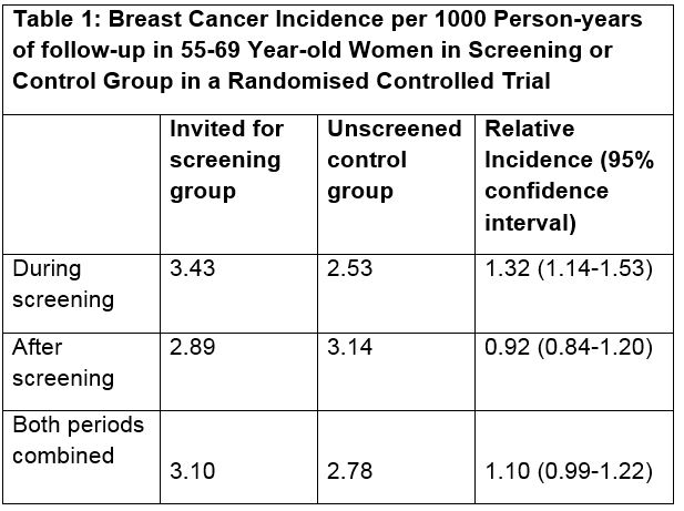
There is continual public debate about the relative benefits and harms to women of taking part in mammographic screening for breast cancer. Table 1 shows data on the incidence of breast cancer among women aged 55-69 years who took part in a randomised controlled trial of the effectiveness of mammographic screening for breast cancer in a western European country. The screening trial lasted for 10 years. After the trial ended women in each of the control and screened groups in this trial were followed for up to 15 years for evidence of death or development of breast cancer. During this follow-up period none of the women in the study was screened.
(a) In one sentence, explain why person-years of follow-up as opposed to persons were used as the denominator in this study? (1 mark)
(b) Which statistical test would be appropriate for analysis of data in this study? (1 mark)
(c) Describe and give one reason for the differences in breast cancer incidence between the screened and control groups during screening, as shown in Table 1. (2 marks)
(d) Describe and give one reason for the differences in breast cancer incidence between the screened and control groups after screening, as shown in Table 1. (2 marks)
(e) Describe and give one reason for the differences in breast cancer incidence between the screened and control groups for both periods combined, as shown in Table 1. (2 marks)
(f) Outline, in no more than two sentences, the unintended adverse consequences to a woman resulting from “overdiagnosis” of breast cancer during screening. (2 marks)
Specimen Section 12
You are carrying out a health needs assessment for immigrants in your country and have been asked to consider the following data available from national mortality statistics:
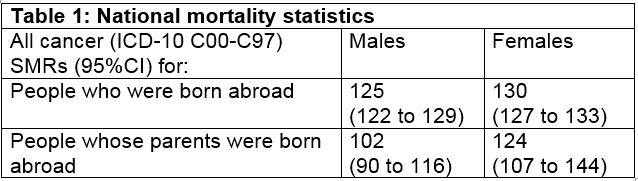
(a) In three bullet points, comment on the figures presented in Table 1 for first generation immigrants. (3 marks)
(b) In three bullet points, comment on the figures presented in Table 1 for second generation immigrants. (3 marks)
Age-adjusted SMRs for cancer in your country were published for second generation immigrant females living in different areas, classified by an area-based socioeconomic deprivation score. For the least deprived areas, the SMR was 112, based on 36 cancer deaths. For the most deprived areas, the SMR was 144, based on 81 cancer deaths.
(c) Derive 95% confidence intervals for each of these SMRs, showing your working. (3 marks)
(d) In one sentence, comment on the association of socioeconomic deprivation with cancer mortality among second generation immigrant females in these published figures. (1 mark)
Model answer to specimen Section 1
| (a) | Catchment population, registered population or population at risk | |||||||
| (b) | Incidence (episodes/spells) ratio = 125/175 = 0.71, or a 29% relative reduction. A ratio measure is preferable to a difference measure as it has no units and we lack a population denominator. | |||||||
| (c) | Population remains constant (in size and demographic structure) over the 2 years. Proportion of all acute attacks presenting in general practice remains constant | |||||||
|
(d) |
The numbers of acute asthma attacks can be considered as Poisson variables with variance = count. The difference between the counts can then be compared to the variance of the difference (variance of the difference = sum of the variances = sum of the counts). A Wald test (SND or z-test) or chi-square test can then be constructed and tested for statistical significance with reference to standard tables. Difference = 175-125 = 50 Var (diff) = 175+125 = 300 SND = z = 50 / sqrt(300) = 50 / 17.32 = 2.89 (which is greater than 1.96) Or…Chisq = z² = 50² / 300 = 8.33 (which is greater than 3.84) |
|||||||
| Another valid approach would be to test the incidence ratio (but this requires use of logarithms to base e (ln), not available on the calculators provided):ln (count1/count2) = ln (count1 – ln (count2) Var (ln(ratio)) = Var (ln(count1)) + Var (ln(count2)) = 1/125 + 1/175Then compare ln(125/175) to Var(ln(ratio)) by SND or Chisq approach as above. |
||||||||
| (e) | Interpret as statistically significant, compare with relatively unchanged prevalence (500 v 450, assuming constant population), consider alternative explanations and suggest comparison with trends in an area outside the CC zone. | |||||||
Model answer to specimen Section 2
| (a) | C | |||||||
| (b) | Improvements in treatment (new drugs, changes in clinical guidelines and practice). Earlier diagnosis (lead-time bias) and detection of slower-growing prevalent cases (length bias), both resulting from increased coverage of breast cancer screening. | |||||||
| (c) | Steady improvement in survival in successive cohorts. Similar trends at all durations of follow-up (1-10 years), consistent with (approximately) proportional hazards. | |||||||
| (d) | Relative reduction in cumulative risk of mortality. Percentage survival needs to be converted to percentage dying (over 5, 10, 15 years) and then express the reduction in mortality risk as a proportion of the original mortality risk. For example, for 5-year data:1980-1984 5-year mortality risk = 100-73 = 27% 1990-1994 5-year mortality risk = 100-88 = 12% Difference 27-12 = 15% Proportional risk reduction 15 / 27 = 0.56 |
|||||||
| (e) | Explain what is meant by overall survival. Describe survival chances for women in each cohort. Note that improvement is sustained throughout 15 years. Comment on the consistency of the proportional risk reductions. | |||||||
Model answer to specimen Section 3
| (a) | 130/691 = 18.8% | |||||||
| (b) | (415/266,542) / (276/253,698) = 1.43 | |||||||
| (c) | Comment on the magnitude and direction of effect ("doubling of risk among multiple births"). 95% probability / confidence that the true value lies within this range (or, if the study was repeated 100 times, expect 95 results within this range). 95% confidence interval does not include 1, so p<0.05 (in fact, lower 95% CL considerably greater that 1, so p can be deduced to be much less than 0.05). | |||||||
| (d) | Cross-sectional survey does not include children who die before 10 years, and the mortality is high among visually impaired children. Thus, lifetime prevalence at 10 will be less than cumulative incidence as measured by the register (assuming that all blind children are registered, which is probably a reasonable assumption). | |||||||
| (e) | Ascertainment of moderate visual impairment at the cross-sectional survey could be more comprehensive, and would pick up (live) cases missed off the register, leading to a higher lifetime prevalence than registered cumulative incidence. | |||||||
Model answer to specimen Section 4
| (a) | 94%, as shown in the table. | |||||||
| (b) | Extra FISH tests | 3,900 | @ | £150 | £ 585,000 extra costs | |||
| HER2-ves untreated | 234 | @ | £25,000 | £5,850,000 costs saved | ||||
| (234 = 6% of 3,900) | £5,265,000 net saving | |||||||
| The saving in unnecessary / ineffective treatment costs clearly outweighs the costs of the additional FISH tests, despite the high PPV in this "strongly positive" IHC group. | ||||||||
| (c) | FISH+ | FISH- | ||||||
| IHC negative | 22,500 | x | 1% | = | 225 | 22,275 | ||
| IHC weak + | 3,600 | x | 50% | = | 1,800 | 1,800 | ||
| IHC strong + | 3,900 | x | 94% | = | 3,666 | 234 | ||
| Total | 30,000 | 5,691 | 24,309 | |||||
| (i) | Sensitivity of IHC strong positive = 3,666/5,691 = 64.4% | |||||||
| (ii) | Sensitivity of IHC strong or weak = 5,466/5,691 = 96.0% | |||||||
| (iii) | Sensitivity of FISH testing (gold standard) = 100% (by definition) | |||||||
| (d) | The current (IHC test) regimen detects 3,666 HER2 positive cases (table above) and costs 30,000 x £40 = £1,200,000 = £1.2M. If all 30,000 specimens were tested with FISH (the gold standard), there would be no need for preliminary IHC testing. All 5,691 HER2 positives would be detected at a cost of 30,000 x £150 = £4,500,000 = £4.5M. Thus, 5,691-3,666 = 2,025 extra cases would be detected at an additional cost of £3.3M. The marginal cost per additional HER2 positive case is: 3.3M/2,025 = £1,629.63 per case. |
|||||||
| (e) | The single most important piece of information would be the benefits (in terms of improved survival and/or quality of life) for HER2-positive women undergoing treatment with trastuzumab. | |||||||
Model answer to specimen Question 5
(a) Ecological study (population-level comparisons).
(b) Regression coefficient represents the slope of the line (increase in asthma prevalence for each 1 per 100,000 increase in swimming pools per unit population). 95%CI does not include zero, therefore the regression/correlation is statistically significant at the 5% level.
(NB: the lower CI of 1.00 should not be confused with a null effect on the relative risk/odds scale.)
(c) Both correlations are positive and statistically significant. The 95%CIs overlap considerably and therefore there is no statistically significant difference between the slopes for each group of children.
(d) How were the cities/centres selected? How were children selected within centres? How was asthma defined and ascertained? What was the source of the swimming pool counts? (1 mark for each of these, to a maximum of 2).
(e) Comparison of proportions, assuming binomial sampling errors, with variance of each proportion var(p) = p(1-p)/n (1 mark for formula, 2 marks for calculation). Calculation of chi-square on 1df from the 2x2 table would be an acceptable alternative.
Model answer to specimen Question 6
(a)
• Derive SEMs as SD /√n for weight in each of the two groups. (1 mark)
• Derive SE(difference) as √[SEM1² + SEM2²] (0.5 mark)
• Derive difference between means by subtraction (D) (0.5 mark)
• 95%CI for difference = D + 1.96*SE(difference) (0.5 mark)
• Comment on statistical significance. (0.5 mark)
(b)
• Sex is a positive confounder in this situation, because at age 10-11, many girls have started their pubertal growth spurt, so girls are taller and heavier than boys;
• children eating school meals are taller and heavier, and are more likely to be girls.
• Adjustment for sex would therefore tend to reduce or possibly reverse the relationship between school meals and height or weight.
(1 mark for each of these points)
(c) Any factors strongly related both to height/weight/BMI and to uptake of school meals (half a mark). Socioeconomic status and ethnic group would be pertinent examples in a UK context (half a mark for a relevant example). To be a confounder it must be related to both eating school meals and children’s height/weight/BMI so candidates needs to justify their factor with that in mind. (1/2 mark)
(d) Examples of potential answers include:
• To measure growth (rather than height) would require longitudinal assessment (or record linkage), whilst also collecting information on potential confounders, including parental heights and weights, family lifestyle, child’s activity patterns.
• Obtain more information on what children are actually eating for lunch (in both groups) and at other times of day (and in holidays). Thus, place the school meals into context, but also address confounding by other aspects of diet.
• Compare schools serving different types of menu at lunchtime, and/or consider a before-and-after comparison if changes are implemented to the school meals.
• Consider a wider range of measurements than just height and weight, such as body mass index or weight-for-height, measures of fat distribution (skinfolds, waist/hip) or fat mass (bioimpedence).
(Up to 3 marks for a well elucidated answer with three key points, or equivalent)
Model answer to specimen Question 7
(a) The principal sources will be death certificates and hospital admission and/or discharge records. Accident & emergency registers and operating theatre records could be used as ancillary sources, particularly for establishing the timing of death in relation to admission and surgery. (1/2 mark for each source)
(b) The principal problems relate to case-definition and record linkage. Any of the following points would gain 1 mark each (to a maximum
of 2):
– An inclusive definition (e.g. any mention of “aortic aneurysm”) will be desirable to identify all cases, but the site of the aneurysm may
not always be recorded or coded (e.g. on death certificates).
– Distinguishing ruptured (emergency) from non-ruptured (elective) aneurysm repairs may not be possible from diagnostic codes.
Reference to procedural codes, theatre records and/or case notes may be required.
– Death certification likely to be less accurate for out-of-hospital deaths, unless confirmed by autopsy.
– In-hospital deaths are likely to appear on both the admissions and death registers. Some method of linking individual records (e.g. patient names, place of residence, date of birth) is required to eliminate double-counting.
– Problems of linkage may arise from cross-border transfers to hospitals outside the health authority area.
(c) The relationship between volume of emergency RAAA repair and post-operative survival:
 - These data suggest that late post-operative mortality, rather than death before, during or immediately after emergency surgery, is the main driver of the differences in survival between hospital catchment areas.
- Although there is an inverse relationship between volume and survival to discharge, this is not seen at 2 days (peri-operative survival).
- Comparison of survival rates for hospitals A, B and C may suggest that factors other than volume of emergency surgery may also be more important. In particular volume of surgery in B is half A yet survival is similar, whilst volume of surgery in B and C are similar yet survival appear different. (But numbers are small)
- This does not support a strong association between quality and volume for emergency vascular surgery, but the weight of evidence
is weak. Policy development would need to be informed by data on a larger number of hospitals. (0.5 mark per point, or reasonable alternate)
(d) Odds ratios are multiplicative, so for 20 minute increment: OR = 0.97 x 0.97 = 0.94, LCL = 0.70 x 0.70 = 0.49, UCL = 1.34 x 1.34 = 1.80. (1 mark for OR, 0.5 mark for UCL and 0.5 mark for LCL)
Thus, a small adverse impact on survival is most likely, but the confidence intervals are wide. Since it is unlikely that prolonging transport time will improve survival, it is the lower 95% limit that is of greater relevance. A halving of the odds of survival cannot be excluded, though this would be balanced against receiving more specialised surgical care (should that be shown in larger studies to enhance survival).
Model answer to specimen Question 8
(a) What mode of transmission of infection do the data in figure 1 indicate? (2 marks)
The epidemic curve indicates an initial point source outbreak followed by secondary faecal-oral spread of infection accounting for the final four cases, on days 15-17. Secondary spread of E. coli O157 infection in nurseries without high standards of hygiene is a high risk.
(b) From table 1, calculate the attack rate for those served beef burger. (1 mark)
In this scenario the attack rate is defined as:
For those served beef burger: number of cases served beef burger/total number of children served beef burger = 40/43 = 93%.
(c) Perform an appropriate statistical test to determine whether or not the difference in attack rate for those served or not served beef burger is statistically significant. (3 marks)
An appropriate test is: either a two-sided chi-squared test of significance on a two by two table with one degree of freedom; or a comparison of two independent proportions.
The formula for the chi-squared test is ∑[(O-E)2/E] for the four cells of the two by two table. For beef burger chi-squared = 49.0, which is a highly significant value with one degree of freedom. This shows that eating beef burger was highly significantly associated with being a case.
Using a comparison of two independent proportions, p1 = 40/43 and p2 = 5/35. The stages are as follows:
1. derive difference in sample proportions p1-p2 = 0.787 or 78.7%
2. derive standard error of the difference in proportions:
S.E (diff) =√ [(p1(1-p1)/n1) + p2(1-p2)/n2] = 0.071 or 7.1%
3. 95% confidence interval = p1-p2 +/- (1.96 X S.E. diff)
= 0.787 +/- 0.0139
= 0.648 – 0.926 or 64.8% - 92.6%
In this case the 95% confidence interval for the difference does not overlap 0, which means that the difference in attack rates for beef burgers is statistically significant at the 5% level, with a 95% chance that the population difference lies between 64.8% and 92.6%.
(d) Further analysis shows that the associations between being served chips or fresh fruit salad and being a case are statistically significant. What four more pieces of information may help you assess whether beef burger, fruit salad or chips was the most likely outbreak vehicle? (4 marks)
Food microbiology (if any is left) may help distinguish contaminated from uncontaminated foodstuffs.
Information on food suppliers may indicate a link with a source already shown to be associated with other similar outbreaks.
Information on the standard of food storage, handling and cooking practices in the nursery kitchen may indicate temperature abuse of high-risk foodstuffs and/or undercooking of high-risk raw foods and/or cross contamination from one foodstuff to another.
Further statistical analysis to adjust for confounders may help, for example chips may only be significantly associated with being a case because most of the children who ate them also ate beef burger.
Model answer to Specimen Question 9
(a) Separately, for both current smokers and never smokers, calculate the relative risk reduction in admissions for heart attack for the period after the introduction of the law banning smoking compared with the period before (2 marks)
Current smokers: (1176 – 1016)/1176 = 13.6% = 14% (1 mark)
Never smokers: (677-537)/677 = 20.7% = 21% (1 mark)
(b) Describe (but do not calculate) what test(s) you might undertake in order to establish whether the different relative risk reduction in admissions for heart attack among current smokers and never smokers was likely to be due to chance. (2 marks)
Two possible answers, either of which is acceptable and would attract two marks:
(i). Calculate 95% confidence intervals for the relative risk reduction for current smokers and never smokers and see if they overlap.
(ii). Do a chi square test (1 degree of freedom) comparing 160/1176 with 140/677
(c) State, in no more than four sentences, two other possible reasons for this reduction. (2 marks)
There are several possible answers. Only two are required and 1 mark should be given for each of a maximum of two correct answers:
- Possible effects of seasonal variations, six month period before was Oct to March ie autumn and winter, and the six month period after was April to Sept, ie spring and summer, one might expect fewer admissions with heart attack in summer than winter.
- The catchment population is not stated and one might assume that it was either the total population of the whole country or a consistent part. However, since these data are from hospital admissions and the denominator population is not mentioned one would need to check that the referral patterns and thus the catchment population had remained unchanged.
- Exclude the possibility of changes in management practices and/or changes in the definition of the condition – seems unlikely in such a short period of time but is possible.
- Exclude the possibility of an increase in deaths from heart attack prior to admission – again seems an unlikely explanation but is possible.
- Any other plausible explanation given.
(d) Assuming that the new law was effective in reducing smoking in public places describe, in no more than two sentences, a potential adverse public health effect of this reduction (1 mark)
Once smoking in public places is banned there is the possibility that more smoking will take place in the home, thus increasing the exposure of children and other non-smokers to second-hand smoke (1 mark).
(e) Cotinine levels in the general population decreased significantly, whereas there was no reduction in cotinine levels in smokers admitted to hospital with heart attack. Explain in no more than three sentences why this might be the case (3 marks)
- Smokers who continued to smoke at the same levels as before the ban continued with the same risk of heart attack and were admitted with heart attack.
- Smokers who reduced their smoking habit, as evidenced by the reduction in the overall reduction in cotinine levels in the general population of smokers, reduced their risk of heart attack and were on average less likely to be admitted with heart attack ie their heart attack was prevented.
- General population estimates of cotinine would also include levels from non-smokers and former smokers, they are also likely to have contributed to the overall population reduction due to their reduced exposure to second-hand smoke.
Model answer to specimen Question 10
(a) Summarize the findings of the data in Table 1. (3 marks)
- The data show that the risk of dying from any cause within the first two years of life for the children in this study given BCG vaccine was lowered to 37% of the risk for unvaccinated children
- The reduction is highly statistically significant: the confidence interval excludes 1.00 by a large margin.
- The same level of risk reduction was found whether or not the data were adjusted for certain confounders.
(b) Suggest two possible reasons why adjustment for covariates did not alter the mortality ratio. (2 marks)
- The covariates were not independent risk factors for all-cause mortality in this region (unlikely to apply to all of them – especially diarrhoea)
- Receipt of BCG vaccination was not related to the covariates in the model (more likely in this instance).
- [A more sophisticated version of the second explanation would be that BCG was related to higher risk in relation to some covariates (e.g. higher risk areas) but was related to lower risk for others (e.g. use of health services). The confounding effects therefore cancelled out when all covariates were included in the model.]
(c) Describe two major biases arising from the design of this study. (4 marks)
Either of the following weaknesses would have the effect of exaggerating any beneficial effect from BCG vaccination on all-cause mortality:
- As in some cases the vaccination status was updated retrospectively when the researchers visited the families, then misclassification of vaccination status could have occurred, particularly in the light of the mother’s practice of discarding parent-held data following the death of her child. This could introduce misclassification bias by incorrectly assigned “unvaccinated “status to dead children who were in fact vaccinated.
- Children could only have received BCG vaccine if they lived long enough to reach the age at which it is offered. Thus, the vaccinated group are selected for longer survival.
(d) What other study design could be used to test whether or not there are non-specific benefits on mortality from BCG vaccination? (1 mark)
- Randomised controlled trial to study vaccine effectiveness
Model answer to specimen Question 11
(a) In one sentence, explain why person-years of follow-up as opposed to persons were used as the denominator in this study? (1 mark)
This study has women with unequal lengths of follow-up, hence person-years is the appropriate denominator to use.
(b) Which statistical test would be appropriate for analysis of data in this study? (1 mark)
A proportional hazards model e.g. that of Cox, would be appropriate because participants are followed up for differing lengths of time.
(c) Describe (1 mark) and give one reason for (1 mark) the differences in breast cancer incidence between the screened and control groups during screening, as shown in table 1. (2 marks)
• During screening the incidence of breast cancer was significantly increased by 32% compared to the control group incidence. The confidence interval shows that there is a 95% chance that the population relative incidence lies between 1.14 and 1.53.
• During screening incidence is expected to increase because of the lead time effect i.e. detection of cancers by screening at an earlier stage than they would ordinarily present.
(d) Describe (1 mark) and give one reason for (1 mark) the differences in breast cancer incidence between the screened and control groups after screening, as shown in table 1.
• After screening stopped the incidence of breast cancer in the screened grouped incidence fell to 92% of the incidence for the unscreened group. The 95% confidence interval overlaps 1, which indicates that the difference was not significant at the 5% level, though the population relative incidence lies between 0.84 and 1.20.
• A reduced incidence after screening stops is expected because breast cancers that ordinarily would have presented at a certain point in time were detected by screening at an earlier point in time.
(e) Describe (1 mark) and give one reason for (1 mark) the differences in breast cancer incidence between the screened and control groups for both periods combined, as shown in table 1. (2 marks)
• When the two periods are combined the incidence in the screening group is 10% higher than for the control group. This difference is of borderline statistical significance at the 5% level because the confidence interval just overlaps 1. The population relative incidence lies between 0.99 and 1.22.
• The increased incidence during the screening period is not completely counterbalanced by the fall after screening stops and therefore screening has resulted in overdiagnosis of breast cancer that would, in the absence of screening, never have presented in the follow-up period: about 10% overdiagnosis suggested by this study.
(f) Outline, in no more than two sentences, the unintended adverse consequences to a woman resulting from “overdiagnosis” of breast cancer during screening. (2 marks)
• Adverse physical effects from unnecessary investigation and treatment.
Adverse psychological effects through believing that she has a potentially lethal cancer when in fact she does not.
Model answer to specimen Question 12
(a) In three bullet points, comment on the figures presented in the table for first generation immigrants (3 marks)
1) Raised to a similar extent in both males and females.
2) Both statistically significantly different from national rates (or narrow CIs = large numbers of deaths).
3) Not consistent with a “healthy migrant effect” or consistent with increased needs for health care among immigrants.
(b) In three bullet points, comment on the figures presented in the table for second generation immigrants (3 marks)
1) Male SMR no longer significantly raised (half mark). The significantly lower than male SMR for first generation migrants as CIs do not overlap (half mark).
2) Female SMR remains elevated to similar extent as for first generation immigrants. (half mark) But with wider CI – not significantly different to first generation figure (half mark).
3) Male-female difference (not formally evaluated for statistical significance) raises the possibility that males and females have integrated differently within the host country/culture (or comment on sex-specific health needs).
Age-adjusted SMRs for cancer in your country were published for second generation immigrant females living in different areas, classified by an area-based socioeconomic deprivation score. For the least deprived areas, the SMR was 112, based on 36 cancer deaths. For the most deprived areas, the SMR was 144, based on 81 cancer deaths.
(c) Derive 95% confidence intervals for each of these SMRs, showing your working. (3 marks)
1 mark for:
95%CI around an observed Poisson count of C is +/- 1.96*sqrt(C) (or +/- 2*sqrt(C))
Least deprived: Observed count = 36 +/- 1.96*6 = 24.24 to 47.76 (allow 24 to 48)
Most deprived: Observed count = 81 +/- 1.96*9 = 63.36 to 98.64 (allow 63 to 99)
I mark for:
The SMRs are ratios of observed to expected numbers of deaths (x100), so
Expected number of deaths = Observed deaths / (SMR/100)
Least deprived: Expected count = 36/1.12 = 32.14
Most deprived: Expected count = 81/1.44 = 56.25
1 mark for:
95%CI for SMRs = range for 100*observed counts / expected count
Least deprived: 100*24.24/32.14 to 100*47.76/32.14 = 75.42 to 148.60
Most deprived: 100*63.36/56.25 to 100*98.64 to 56.25 = 112.64 to 175.36
(d) In one sentence, comment on the association of socioeconomic deprivation with cancer mortality among second generation immigrant females in these published figures. (1 mark)
The confidence intervals overlap considerably (each CI includes the central SMR estimate for the other group), so there is no statistically significant effect of area deprivation score on the excess cancer mortality among female second generation immigrants
Note:
If the confidences intervals have been incorrectly derived give credit (1 mark) if there is a correct interpretation of a wrong answer.
